Stacking of a simulated CMB temperature map

import numpy as np
import healpy as hp
import matplotlib.pyplot as plt

from cmbstack import StackingPipeline, maps, stacking

fname = 'base_plikHM_TTTEEE_lowl_lowE_lensing.minimum.theory_cl'

Run Peak Stacking Pipeline

The first step is to create a StackingPipeline object. This tutorial shows the stacking procedure for a simulated CMB temperature map from a theoretical power sepctrum using StackingPipeline.from_cl. We can use from_fits or from_map when working with a real or pre-simulated map.

pipeline = StackingPipeline.from_cl(fname, nside=1024, seed=42)

The stacked peak can then be obtained using the run method:

stacked_result = pipeline.run(size_deg=10, reso_arcmin=3, profile=True,threshold=3,n_peaks=None)

stacked_result stores every intermediate product as an attribute:

Attribute	Content
pipeline.map	Raw simulated map
pipeline.normalized	Normalised map (units of \(\sigma\))
pipeline.positions	Peak positions \((θ, φ)\) in radians
pipeline.patches	List of 2D gnomonic patches
pipeline.stacked	Mean stacked 2D image
pipeline.radius	Radial bin centres (arcmin)
pipeline.profile	Mean temperature per radial bin

Below we describe how every intermediate product is obtained by running manually the functions that pipeline.run()calls internally.

1. Load theoretical spectrum — maps.load_cl

The input file contains the power spectrum as \(D_\ell^{TT}\):

\[D_\ell \equiv \frac{\ell(\ell+1)}{2\pi} C_\ell\]

load_cl reads columns \((\ell, D_\ell)\) and converts to \(C_\ell\):

\[C_\ell = \frac{2\pi}{\ell(\ell+1)} D_\ell, \qquad C_0 = C_1 = 0\]

cl = maps.load_cl(fname)
type(cl)

numpy.ndarray

2. Simulate a Sky Map — maps.simulate_map

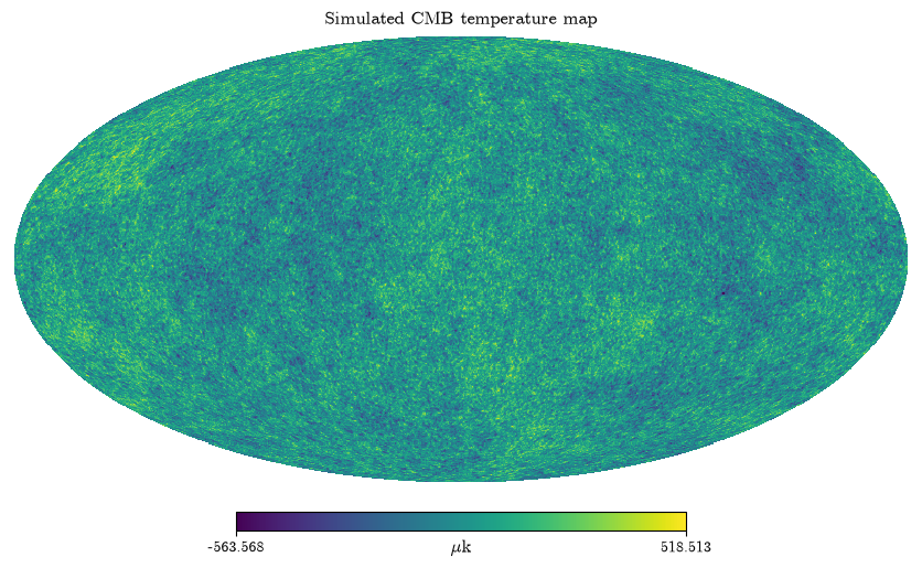
A Gaussian random realization is drawn by sampling spherical harmonic coefficients \(a_{\ell m}\) with variance \(C_\ell\):

\[T(\hat{n}) = \sum_{\ell,m} a_{\ell m} \, Y_{\ell m}(\hat{n}), \qquad \langle |a_{\ell m}|^2 \rangle = C_\ell\]

This calls healpy.synfast internally. An optional seed makes runs reproducible.

sim_map = maps.simulate_map(cl,nside=1024,seed=42)
hp.mollview(sim_map,title='Simulated CMB temperature map',unit=r'$\mu$k')

print("mean:", np.nanmean(sim_map))
print("std: ", np.nanstd(sim_map))       # expect ~100 (μK)
print("min/max:", np.nanmin(sim_map), np.nanmax(sim_map))

mean: -1.0000346790661752e-06
std:  112.69465336088571
min/max: -587.8310256096638 535.185661970055

3. Normalise the Map — maps.normalize_map

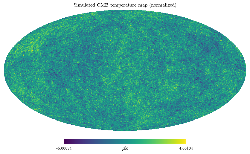
Before peak detection, the map is standardised so that thresholds have a clear statistical meaning:

\[T_{\text{norm}}(\hat{n}) = \frac{T(\hat{n}) - \langle T \rangle}{\sigma}\]

After this step the map has mean \(\approx 0\) and standard deviation \(= 1\), so peaks are measured in units of \(\sigma\).

map_norm = maps.normalize_map(sim_map)
hp.mollview(map_norm,title='Simulated CMB temperature map (normalized)',unit=r'$\mu$k')

print("mean:", np.nanmean(map_norm))      # expect ~0 (monopole removed)
print("std: ", np.nanstd(map_norm))       # expect ~1
print("min/max:", np.nanmin(map_norm), np.nanmax(map_norm)) # sigma units

mean: -3.700743415417188e-17
std:  0.9999999999999999
min/max: -5.216139427016107 4.748988944987899

4. Detect Peaks — stacking.find_peaks

Local maxima are identified with healpy.hotspots: a pixel is a maximum if its value exceeds every immediate HEALPix neighbour. Peaks are filtered by a significance threshold \(\nu\) (default \(\nu = 3\sigma\)) and optionally capped at the \(N\) highest:

\[\text{Peaks} = \{\hat{n}_p \in \text{Maxima} \mid T_{\text{norm}}(\hat{n}_p) > \nu\}\]

Returns sky positions as \((θ, φ)\) pairs in radians.

peak_positions = stacking.find_peaks(map_norm,1024,threshold=3,n_peaks=None)
print(f"Found {len(peak_positions)} peaks above 3 sigma threshold.")

Found 2588 peaks above 3 sigma threshold.

5. Extract Patches — stacking.extract_patches

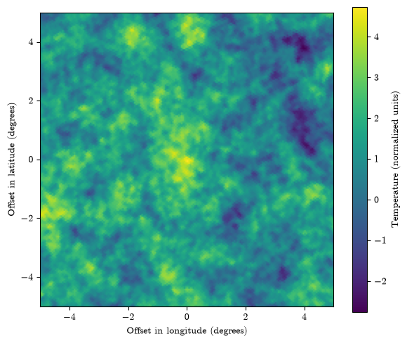
For each peak a square patch is cut using a gnomonic (tangent-plane) projection centred on \(\hat{n}_p\). Every patch shares the same fixed pixel grid (side length size_deg, pixel scale reso_arcmin), so the centre pixel always corresponds to the peak itself and patches can be co-added directly.

patches = stacking.extract_patches(map_norm,peak_positions,size_deg=10,reso_arcmin=3)

The following figure shows an example of an obtained patch

plt.figure(figsize=(6,5))
ny, nx = patches[0].shape
half_x = 0.5 * nx * 3 / 60.0
half_y = 0.5 * ny * 3 / 60.0
extent = [-half_x, half_x, -half_y, half_y]

plt.imshow(patches[0], origin="lower", extent=extent)
plt.xlabel("Offset in longitude (degrees)")
plt.ylabel("Offset in latitude (degrees)")
plt.colorbar(label="Temperature (normalized units)")
plt.tight_layout()
plt.show()

6. Stack — stacking.stack_patches

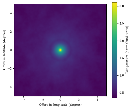
Patches are averaged pixel-by-pixel:

\[S = \frac{1}{N} \sum_{i=1}^{N} P_i\]

Incoherent noise averages towards zero; the coherent central profile survives.

stacked = stacking.stack_patches(patches)

ny, nx = stacked.shape
half_x = 0.5 * nx * 3 / 60.0
half_y = 0.5 * ny * 3 / 60.0
extent = [-half_x, half_x, -half_y, half_y]

plt.figure(figsize=(6, 5))
plt.imshow(stacked,origin='lower', extent=extent)
plt.xlabel('Offset in longitude (degrees)')
plt.ylabel('Offset in latitude (degrees)')
plt.colorbar(label=r'Temperature (normalized units)')
plt.show()

7. Radial Profile — stacking.radial_profile

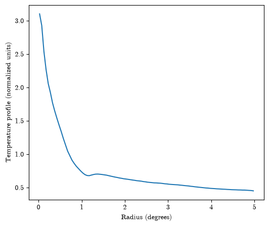
The 2D stacked image is collapsed to a 1D profile by azimuthal averaging in concentric annuli about the centre. Returns bin-centre radii in arcminutes and the mean temperature in each annulus.

radius, profile = stacking.radial_profile(stacked,reso_arcmin=3)

radius_deg = radius / 60.0
plt.figure(figsize=(6,5))
plt.plot(radius_deg,profile)
plt.xlabel('Radius (degrees)')
plt.ylabel(r'Temperature profile (normalized units)')
plt.show()

Saving/loading the map – maps.save_map/maps.load_map

These functions wrap the healpy FITS readers for convenient saving/loading of the simulated maps.

maps.save_map("map_norm.fits", map_norm,overwrite=True)

setting the output map dtype to [dtype('float64')]

m = maps.load_map("map_norm.fits", field=0)